LINEAR REGRESSION
How linear regression fits a best-fit line by minimizing squared error, when its assumptions hold, and why it remains the default baseline.
Part of: AILinear regression is a supervised machine learning model that predicts a continuous number — price, demand, temperature, revenue — by fitting a straight line (in one feature) or a hyperplane (in many features) from inputs to the target.
It is not “just a beginner algorithm.” It is the reference baseline almost every serious project should beat before claiming that a more complex model is worth the cost, complexity, and opacity.
How Linear Regression Makes a Prediction
- Collect paired examples: features X and a numeric target y.
- Choose coefficients (slope(s) and intercept) that minimize total prediction error on the training set.
- For a new row of features, compute
ŷ = β₀ + β₁x₁ + β₂x₂ + …
and treat ŷ as the prediction.
In one dimension that equation is the familiar line y = mx + b. In higher dimensions each coefficient answers a business question when features are scaled and not collinear: holding other inputs fixed, how much does the target change when this feature moves by one unit?
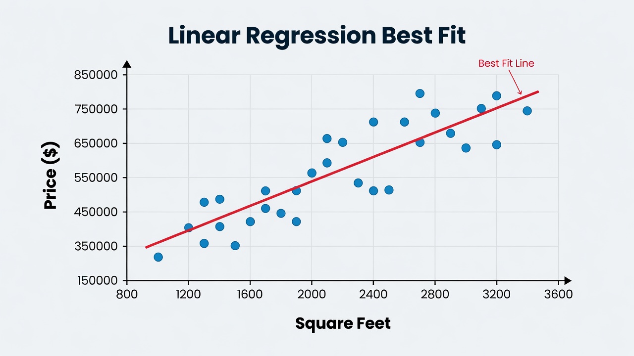
Points = observations. Line = model. Vertical gaps = residuals the algorithm works to shrink.
Ordinary Least Squares (What “Best Fit” Means)
The standard fit is ordinary least squares (OLS):
- Residual for each point: eᵢ = yᵢ − ŷᵢ (vertical error).
- Loss: Σ eᵢ² (sum of squared residuals).
- Solution: coefficients that minimize that loss.
| Choice | Why it matters |
|---|---|
| Vertical residuals | Error is in the target we care about predicting |
| Squares | Large mistakes dominate the fit; math stays closed-form |
| Closed form | Fast, deterministic training — no learning-rate theater for the basic model |
There are variants (ridge, lasso, elastic net) that add regularization when you have many features or multicollinearity. They keep the linear form but shrink or zero coefficients to improve generalization — always validate with model evaluation on a holdout set.
Watch: Linear Regression Explained Visually
VIDEO — STATQUEST (JOSH STARMER)
Short visual walkthrough of how the line settles where total squared error is smallest.
Assumptions (and What to Do When They Break)
Classical OLS theory leans on several assumptions. Production teams care less about textbook purity and more about whether residuals look catastrophic.
| Assumption | Intuition | If badly violated |
|---|---|---|
| Linearity | Target moves roughly straight with features | Add transforms, interactions, or switch to decision trees / non-linear models |
| Independence | Rows are not secretly duplicated or time-chained without care | Use time-aware splits; clustered or panel methods |
| Homoscedasticity | Residual spread is roughly constant | Weighted least squares, transforms, or different model class |
| Normal residuals | Needed for classic confidence intervals | Prediction can still work; be careful with p-value theater |
| No perfect multicollinearity | Features are not exact linear copies | Drop or combine features; regularize |
Practical check: plot residuals vs fitted values and vs key features after fitting. Patterns (curves, funnels, clumps) tell you the line is the wrong shape — not that “regression is dead.”
Strengths and Limitations
Strengths
- Extremely fast to train and serve.
- Coefficients are often directly interpretable (with scaling and domain care).
- Excellent baseline: if a fancy model barely beats OLS, prefer the simple model in production.
- Minimal hyperparameter surface for basic OLS.
Limitations
- Misses curves, thresholds, and interactions unless you engineer features by hand.
- Outliers can tilt the whole line (squared loss is sensitive).
- Unstable coefficients when features are highly correlated.
- Not the right primary tool for images, free text, or audio as raw inputs.
Linear Regression vs Trees vs Neural Nets
| Need | Prefer |
|---|---|
| Continuous target, roughly linear, need speed + explainability | Linear regression |
| Tabular data with interactions, mixed types, rule-like behavior | Decision trees → forests / boosting |
| Unstructured primary signal (vision, language, audio) | Neural nets |
| Must prove the model generalizes | Always: holdout metrics via model evaluation |
Trees and linear models are complements: many teams ship a linear baseline, a tree ensemble challenger, and only then discuss deep learning for tabular data.
When to Use It (and When Not To)
Use linear regression when:
- The target is a continuous number (or a well-justified transform of one).
- Stakeholders need to understand direction and rough magnitude of effects.
- You need a baseline before spending weeks on a complex pipeline.
- Data is moderate-sized and mostly structured/numeric.
Be careful when:
- The relationship is clearly non-linear or piecewise (thresholds, “only if both conditions”).
- Extreme outliers dominate the loss and cannot be winsorized with domain approval.
- You need human-readable paths rather than coefficients (trees win for policy narratives).
- The job is pure classification without a probabilistic linear link (logistic regression is the sibling for binary outcomes — different loss, same linear-in-features spirit).
Practical Workflow: Baseline First
Before you train a 500-tree booster or a small neural net:
- Fit a simple linear regression (or regularized linear model).
- Read coefficients with a domain expert; fix data leaks and broken units.
- Inspect residual plots; engineer a few transforms only if residuals demand it.
- Record holdout RMSE / MAE / R² (model evaluation).
- Only then try trees or other models — and keep the linear model if the gain is tiny.
Many “advanced” projects discover the linear baseline was ~90% as good as the complex model and far easier to monitor, explain, and debug.
Real-World Uses
- Pricing & valuation — real estate, used assets, simple insurance components
- Demand & planning — inventory, staffing, capacity
- Finance & ops — forecasts, sensitivity analysis, “what-if” coefficients
- Science & engineering — calibration, controlled experiments with continuous outcomes
Whenever the output is a number and the first question is “is there any linear signal at all?”, start here.
Related Reading
- Building Your First ML Model — house-price style first build
- 5 Essential Machine Learning Algorithms Explained Simply — linear models next to trees and peers
- Decision Trees — when non-linear tabular structure takes over
- Machine Learning — the broader map
- Model Evaluation — how to know if the line actually generalizes
Linear regression remains the measuring stick of applied ML: not always the final model, but the model you must understand to know whether everything else is progress — or theater.
Part of the knowledge graph at The Best Blog Ever — reference definitions for ideas that matter.